Summary
This project started as a way for me to better understand how propellers behave under different operating conditions — specifically thrust and torque as functions of airspeed and RPM. I wanted to build a model that could estimate performance values purely from geometry and physics-based calculations, without relying on expensive simulations or wind tunnel testing. The final result is a MATLAB-based script that uses blade element momentum theory (BEMT), along with a custom geometry model, to predict thrust and torque across a range of propellers and conditions. I also built a system to compare these predictions to APC’s ANSYS simulation data to see where the model succeeded and where it broke down.
Geometry Modelling
I based all geometry on APC propellers, since they provide a consistent pitch-diameter naming system and have solid simulation data available for validation. My goal was to recreate a mathematical model of their typical blade shape.
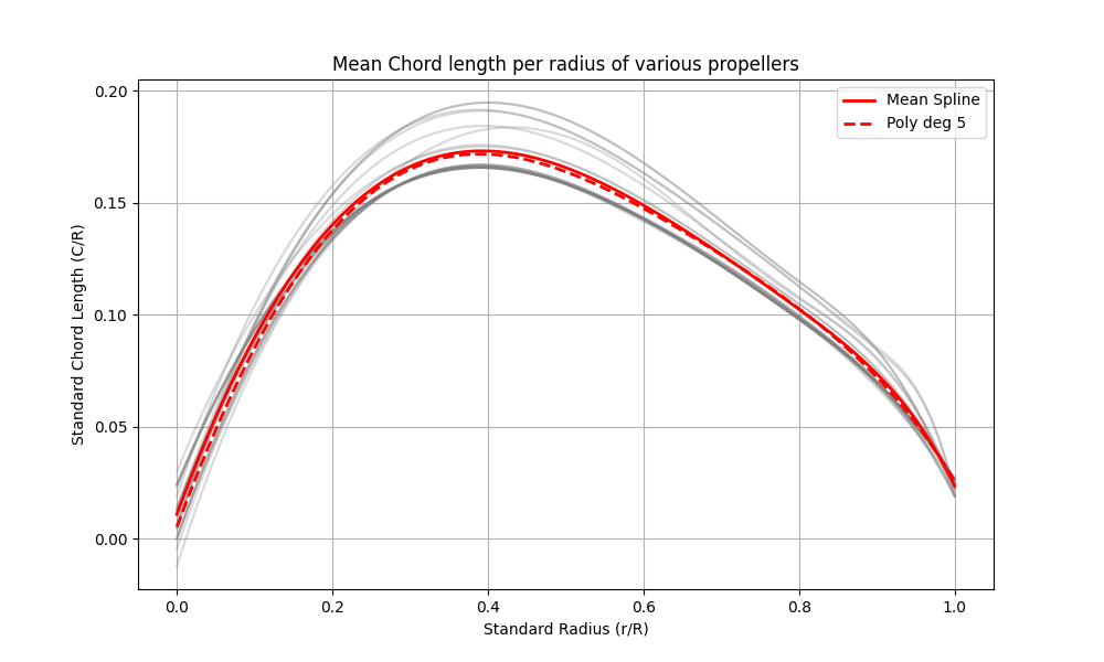
To do that, I pulled a large sample of chord distributions from different APC propellers — basically measuring how the width of the blade changes from root to tip. After analyzing that data, I wrote a script to find the average normalized chord shape across dozens of propellers. That gave me a polynomial chord distribution that could be scaled based on the given diameter.
For each blade, I recreated a 2D representation by slicing it into radial sections and assigning the appropriate chord length at each point. From there, I could input any diameter and pitch, and the model would generate a full radial profile.
Inflow and Axial Velocity Convergence
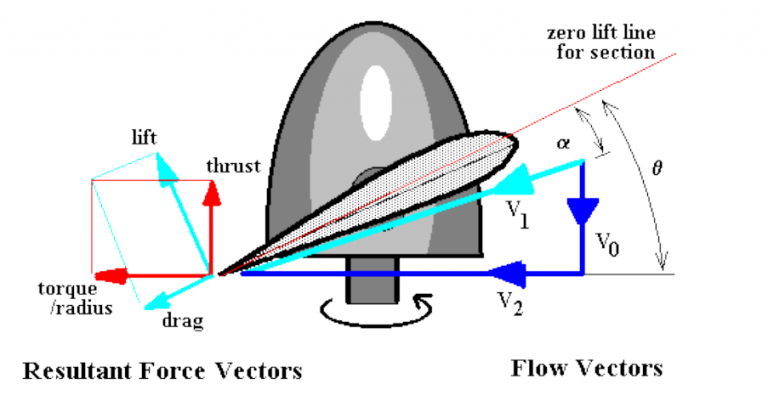
The thrust and torque calculations themselves are based on BEMT with some iterative tweaks. The heart of the code runs through about 30 radial stations per blade, estimating local velocities, angles of attack, and aerodynamic forces.
One of the trickier parts was handling the axial (inflow) and tangential (swirl) velocity components. These aren’t constants — they’re influenced by the blade’s own motion and need to be solved iteratively. For each radial point, the script starts with a guess for the inflow factor a and swirl factor b, then adjusts them until they converge to stable values. This requires computing local induced velocities, finding the angle of attack, calculating lift and drag coefficients, and then comparing the result to what momentum theory predicts. If they don’t match, the script updates a and b and loops again.
The result is a pair of integrated values for total thrust and torque. I found that around 30 stations was a good balance between accuracy and speed.
Data Verification and Comparison
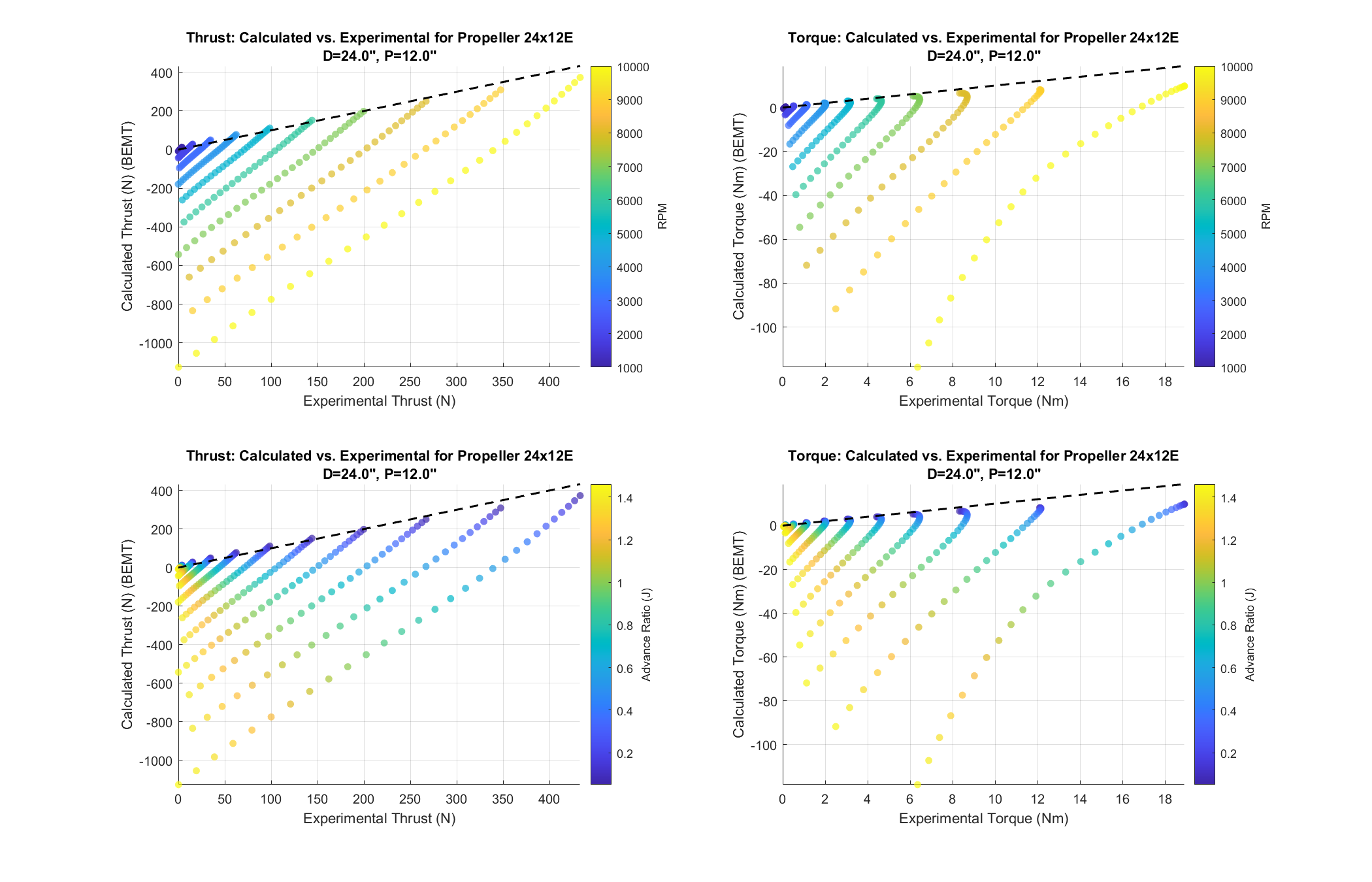
After building the model, I wanted to see how close it came to reality. APC publishes ANSYS-generated thrust and torque values across various RPMs and incoming airspeeds, which gave me a great baseline to test against.
I wrote another script to automatically pull that data and compare it to my model’s output. The comparison showed some clear trends: at low RPMs, the model tended to slightly overpredict thrust, but as RPM increased, it shifted to underpredicting — especially for torque. The torque underprediction became particularly noticeable at high RPMs, which may be due to simplifications in the drag modeling or swirl assumptions.
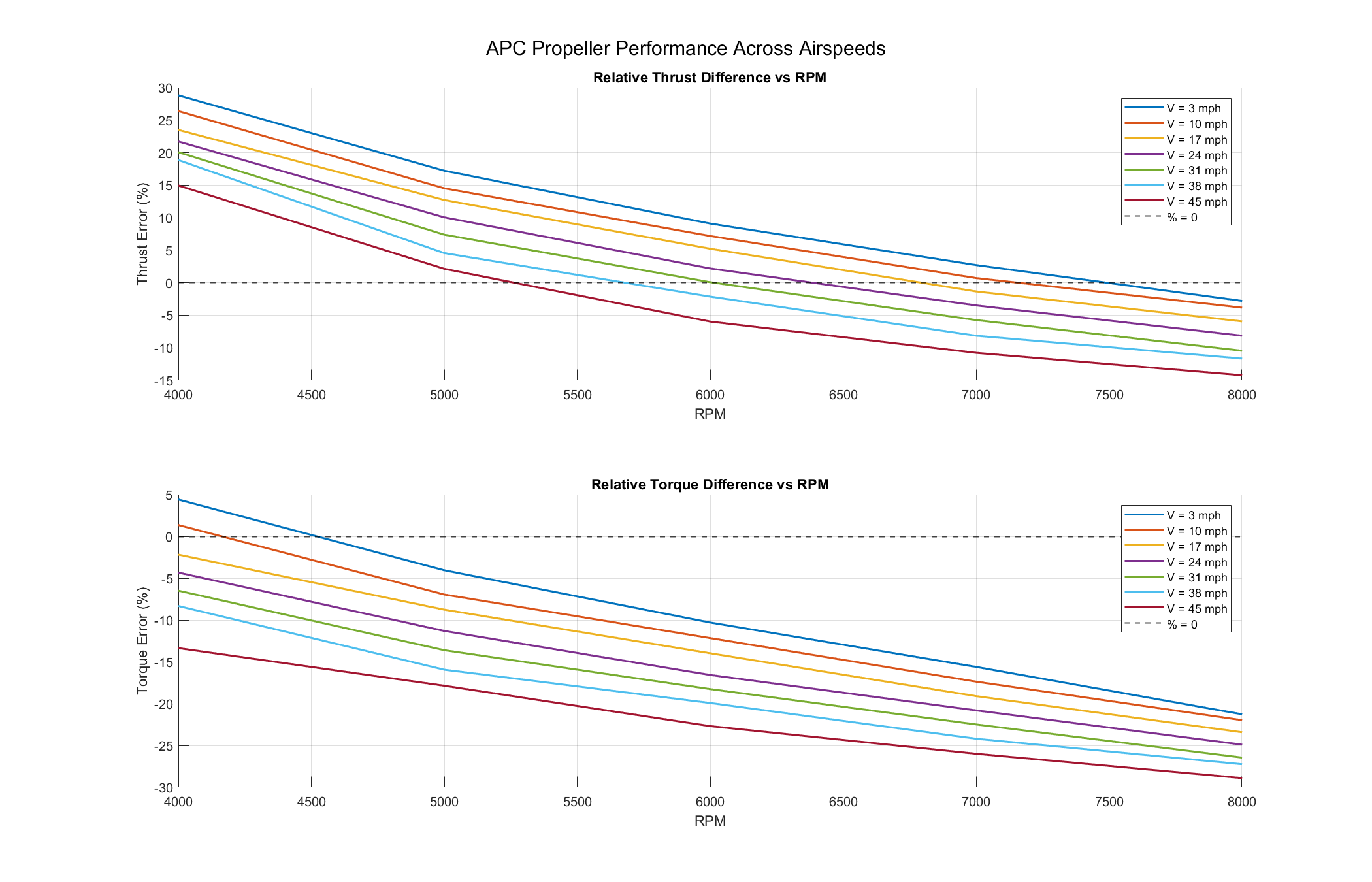
I also tested different incoming airspeeds and plotted results against both RPM and advance ratio. It became clear that advance ratio had the bigger impact on prediction error — likely because higher advance ratios amplify any inaccuracies in blade angle or drag estimation. RPM was still useful to look at, but didn’t explain as much of the difference.
Detailed Airfoil Simulation
Initially, the model used a pretty basic aerodynamic assumption: lift coefficient (Cl) was linear with angle of attack, and drag coefficient (Cd) followed a parabolic curve. This worked fine for quick simulations, but I had to clamp both Cl and Cd once the angle of attack passed a reasonable stall limit — around ±15 degrees. It simplified things, but also introduced some serious limitations, especially at higher advance ratios where those approximations start to break down.
After noticing that advance ratio was the biggest contributor to error — especially in underpredicting torque at high RPMs — I decided to refine the airfoil model. My first approach involved running detailed simulations in XFLR5 to generate Cl and Cd data across a wide range of angles of attack and Reynolds numbers. I set up a batch process to sweep through relevant conditions and generate tabulated data for each, which the MATLAB model could then interpolate during runtime. After further research, however, I realized that the 2D airfoil XFLR5 simulated did not take into account the 3D coriolis fluid flow affecting it. As a result, I was predicting airfoil stall earlier than exeperimental data suggested.
This gave much more realistic force predictions, especially for off-design operating points. While the model still tended to perform better at lower advance ratios, the accuracy at higher RPMs noticeably improved. The torque underprediction issue became less severe, and the transition from over- to under-prediction smoothed out. It wasn’t perfect, but it showed that using real aerodynamic data made a significant difference — and reinforced that a one-size-fits-all Cl/Cd model doesn’t hold up well when the propeller is pushed away from its design point.